Text-Mining the DLD Conference 2014

Once a year, the cosmopolitan digital avantgarde gathers in Munich to listen to keynotes on topics all the way from underground gardening to digital publishing at the DLD, hosted by Hubert Burda. In the last years, I did look at the event from a network analytical perspective. This year, I am analyzing the content, people were posting on Twitter in order to make comparisons to last years’ events and the most important trends right now.

To do this in the spirit of Street Fighting Trend Research, I limited myself to openly available free tools to do the analysis. The data-gathering part was done in the Google Drive platform with the help of Martin Hawksey’s wonderful TAGS script that is collecting all the tweets (or almost all) to a chosen hashtag or keyword such as “#DLD14” or “#DLD” in this case. Of course, there can be minor outages in the access to the search API, that appear as zero lines in the data – but that’s not different to data-collection e.g. in nanophysics and could be reframed as adding an extra challenge to the work of the data scientist 😉 The resulting timeline of Tweets during the 3 DLD days from Sunday to Tuesday looks like this:

Twitter Buzz for #DLD14

You can clearly see three spikes for the conference days, the Monday spike being a bit higher than the first. Also, there is a slight decline during lunch time – so there doesn’t seem to be a lot food tweeting at the conference. To produce this chart (in IPython Notebook) I transformed the Twitter data to TimeSeries objects and carefully de-duplicated the data. In the next step, I time shifted the 2013 data to find out how the buzz levels differed between last years’ and this years’ event (unfortunately, I only have data for the first two days of DLD 2013.

DLD14_Buzz_Comp_Comparison

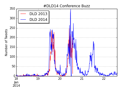
The similarity of the two curves is fascinating, isn’t it? Although there still are minor differences: DLD14 began somewhat earlier, had a small spike at midnight (the blogger meeting perhaps) and the second day was somewhat busier than at DLD13. But still, not only the relative, but also the absolute numbers were almost identical.

Now, let’s take a look at the devices used for sending Tweets from the event. Especially interesting is the relation between this years’ and last years’ percentages to see which devices are trending right now:

DLD14_Clients

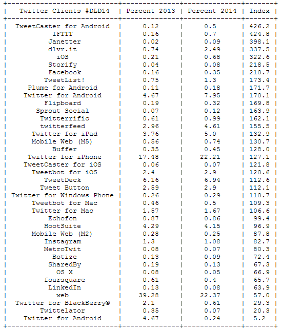
The message is clear: mobile clients are on the rise. Twitter for Android has almost doubled its share between 2013 and 2014, but Twitter for iPad and iPhone have also gained a lot of traction. The biggest losers is the regular Twitter web site dropping from 39 per cent of all Tweets to only 22 per cent.

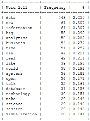
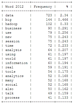
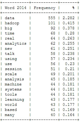
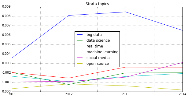
The most important trending word is “DLD14”, but this is not surprising. But the other trending words allow deeper insights into the discussions at the DLD: This event was about a lot of money (Jimmy Wales billion dollar donation), Google, Munich and of course the mobile internet:

DLD14_Words

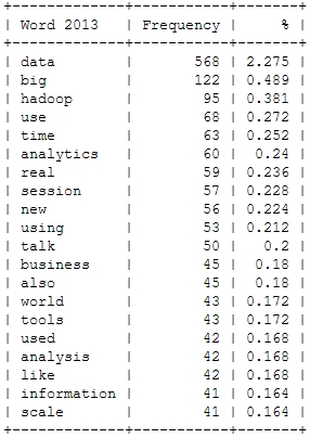
Compare this with the top words for DLD 2013:

DLD13_Words

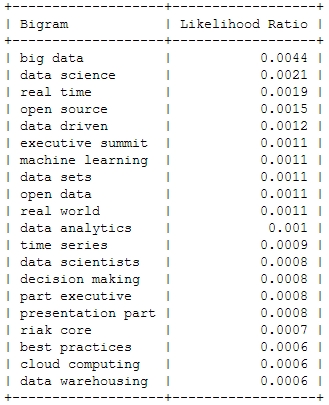
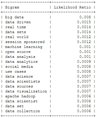
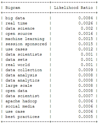
Wait – “sex” among the 25 most important words at this conference? To find out what’s behind this story, I analyzed the most frequently used bigrams or word combinations in 2013 and 2014:

DLD13_Bigrams DLD14_Bigrams

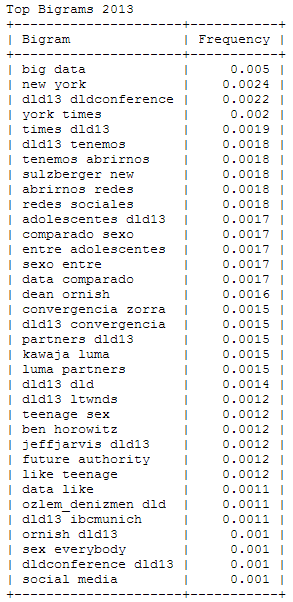
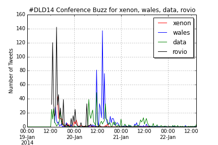
With a little background knowledge, it clearly shows that 2013’s “sex” is originating from a DJ Patil quote comparing “Big Data” (the no. 1 bigram) with “Teenage Sex”. You can also find this quotation appearing in Spanish fragments. Other bigrams that were defining the 2013 DLD were New York (Times) and (Arthur) Sulzberger, while in 2014 the buzz focused on Jimmy Wales, Rovio and the new Xenon processor and its implications for Moore’s law. In both years, a significant number of Tweets are written in Spanish language.

DLD14_Buzzwords_Comp

UPDATE: Here’s the  IPython Notebook with all the code, this analysis has been based on.

Trending Topics at Strata Conferences 2011-2014

To fill the gap until this year’s Strata Conference in Santa Clara, I thought of a way to find out trends in big data and data science. As this conference should easily be the leading edge gathering of practitioners, theorists and followers of big data analytics, the abstracts submitted and accepted for Strataconf should give some valuable input. So, I collected the abstracts from the last Santa Clara Strata conferences and applied some Python nltk magic to it – all in a single IPython Notebook, of course.

Here’s a look at the resulting insights. First, I analyzed the most frequent words, people used in their abstracts (after excluding common English language stop words). As a starter, here’s the Top 20 words for the last four Strata conferences:

Strata_Words_2011 Strata_Words_2012 Strata_Words_2013 Strata_Words_2014

This is just to check, whether all the important buzzwords are there and we’re measuring the right things here: Data – check! Hadoop – check! Big – check! Business – check! Already with this simple frequency count, one thing seems very interesting: Hadoop didn’t seem to be a big topic in the community until 2012. Another random conclusion could be that 2011 was the year where Big Data really was “new”. This word loses traction in the following years.

And now for something a bit more sophisticated: Bigrams or frequently used word combinations:

2011
Strata_Bigrams_2011
2012
Strata_Bigrams_2012
2013
Strata_Bigrams_2013
2014
Strata_Bigrams_2014

Of course, the top bigram through all the years is “big data”, which is not entirely unexpected. But you can clearly see some variation among the Top 20. Looking at the relative frequency of the mentions, you can see that the most important topic “Big Data” will probably not be as important in this years conference – the topical variety seems to be increasing:

Strata_Bigrams

Looking at some famous programming and mathematical languages, the strong dominance of R seems to be broken by Python or IPython (and its Notebook environment) which seems to have established itself as the ideal programming tool for the nerdy real-time presentation of data hacks. \o/

Strata_Lang

Another trend can be seen in the following chart: Big Data seems to become more and more faceted over the years. The dominant focus on business applications of data analysis seems to be over and the number of different topics discussed on the conference seems to be increasing:

Strata_Fields

Finally, let’s take a more systematic look at rising topics at Strata Conferences. To find out which topics were gaining momentum, I calculated the relative frequencies of all the words and compared them to the year before. So, here’s the trending topics:

Strata_Trends_2012 Strata_Trends_2013 Strata_Trends_2014

These charts show that 2012 was indeed the “Hadoop-Strata” where this technology was the great story for the community, but also the programming language R became the favorite Swiss knife for data scientists. 2013 was about applications like Hive that run on top of Hadoop, data visualizations and Google seemed to generate a lot of buzz in the community. Also, 2013 was the year, data really became a science – this is the second most important trending topic. And this was exactly the way, I experienced the 2013 Strata “on the ground” in Santa Clara.

What will 2014 bring? The data suggests, it will be the return of the hardware (e.g. high performance clusters), but also about building data architectures, bringing data know-how into organizations and on a more technical dimension about graph processing. Sounds very promising in my ears!

Identifying trends in the German Google n-grams corpus (Tutorial)

A lot of people still have a lot of respect for Hadoop and MapReduce. I experience it regularly in workshops with market researchers and advertising people. Hadoop’s image is quite comparable with Linux’ perceived image in the 1990s: a tool for professional users that requires a lot of configuration. But in the same way, there were some user-friendly distributions (e.g. Suse), there are MapReduce tools that require almost no configuration.

One favorite example is the ease and speed, you can do serious analytical work on the Google n-grams corpus with Hive on Amazon’s Elastic MapReduce platform. I adapted the very helpful code from the AWS tutorial on the English corpus to find out the trending German words (or 1-grams) for the last century. You need to have an Amazon AWS account and valid SSH keys to connect to the machines you are running the MapReduce programs on (here’s the whole hive query file).

  • Start your Elastic MapReduce cluster on the EMR console. I used 1 Master and 19 slave nodes. Select your AWS ssh authorization key. Remember: from this moment on, your cluster is generating costs. So, don’t forget to terminate the cluster after the job is done!
  • If your Cluster has been set-up and is running, note the Master-Node-DNS. Open a SSH client (e.g. Putty on Windows or ssh on Linux) and connect to the master node with the ssh key. Your username on the remote machine is “hadoop”.
  • Start “hive” and set some useful defaults for the analytical job:

    set hive.base.inputformat=org.apache.hadoop.hive.ql.io.HiveInputFormat;
    set mapred.min.split.size=134217728;

  • The first code snippet connects to the 1-gram dataset which resides on the S3 storage:

    CREATE EXTERNAL TABLE german_1grams (
    gram string,
    year int,
    occurrences bigint,
    pages bigint,
    books bigint
    )
    ROW FORMAT DELIMITED FIELDS TERMINATED BY '\t'
    STORED AS SEQUENCEFILE
    LOCATION 's3://datasets.elasticmapreduce/ngrams/books/20090715/ger-all/1gram/';

  • Now, we can use this database to perform some operations. The first step is to normalize the database, e.g. to transform all words to lower case and remove 1-grams that are no proper words. Of course you could further refine this step to remove stopwords or reduce the words to their stems by stemming or lemmatization.

    CREATE TABLE normalized (
    gram string,
    year int,
    occurrences bigint
    );

    And then we populate this table:

    INSERT OVERWRITE TABLE normalized
    SELECT
    lower(gram),
    year,
    occurrences
    FROM
    german_1grams
    WHERE
    year >= 1889 AND
    gram REGEXP "^[A-Za-z+'-]+$";

  • The previous steps should run quite fast. Here’s the step that really need to be run on a multi-machine cluster:

    CREATE TABLE by_decade (
    gram string,
    decade int,
    ratio double
    );

    INSERT OVERWRITE TABLE by_decade
    SELECT
    a.gram,
    b.decade,
    sum(a.occurrences) / b.total
    FROM
    normalized a
    JOIN (
    SELECT
    substr(year, 0, 3) as decade,
    sum(occurrences) as total
    FROM
    normalized
    GROUP BY
    substr(year, 0, 3)
    ) b
    ON
    substr(a.year, 0, 3) = b.decade
    GROUP BY
    a.gram,
    b.decade,
    b.total;

  • The final step is to count all the trending words and export the data:

    CREATE TABLE result_decade (
    gram string,
    decade int,
    ratio double,
    increase double );

    INSERT OVERWRITE TABLE result_decade
    SELECT
    a.gram as gram,
    a.decade as decade,
    a.ratio as ratio,
    a.ratio / b.ratio as increase
    FROM
    by_decade a
    JOIN
    by_decade b
    ON
    a.gram = b.gram and
    a.decade - 1 = b.decade
    WHERE
    a.ratio > 0.000001 and
    a.decade >= 190
    DISTRIBUTE BY
    decade
    SORT BY
    decade ASC,
    increase DESC;

  • The result is saved as a tab delimited plaintext data file. We just have to find out its correct location and then transfer it from the Hadoop HDFS file system to the “normal” file system on the remote machine and then transfer it to our local computer. The (successful) end of the hive job should look like this on your ssh console:
    EMR_finish
    The line “Deleted hdfs://x.x.x.x:9000/mnt/hive_0110/warehouse/export” gives you the information where the file is located. You can transfer it with the following command:

    $ hdfs dfs -cat /mnt/hive_0110/warehouse/export/* > ~/export_file.txt

  • Now the data is in the home directory of the remote hadoop user in the file export_file.txt. With a secure file copy program such as scp or WinSCP you can download the file to your local machine. On a Linux machine, I should have converted the AWS SSH key in the Linux format (id_rsa and id_rsa.pub) and then added. With the following command I could download our results (replace x.x.x.x with your IP address or the Master-Host-DNS):

    $ scp your_username@x.x.x.x:export_file.txt ~/export_file.txt

  • After you verified that the file is intact, you can terminate your Elastic MapReduce instances.

As a result you get a large text file with information on the ngram, decade, relative frequency and growth ratio in comparison with the previous decade. After converting this file into a more readable Excel document with this Python program, it looks like this:
ngrams_results

Values higher than 1 in the increase column means that this word has grown in importance while values lower than 1 means that this word had been used more frequently in the previous decade.

Here’s the top 30 results per decade:

  • 1900s: Adrenalin, Elektronentheorie, Textabb, Zysten, Weininger, drahtlosen, Mutterschutz, Plazenta, Tonerde, Windhuk, Perseveration, Karzinom, Elektrons, Leukozyten, Housz, Schecks, kber, Zentralwindung, Tarifvertrags, drahtlose, Straftaten, Anopheles, Trypanosomen, radioaktive, Tonschiefer, Achsenzylinder, Heynlin, Bastimento, Fritter, Straftat
  • 1910s: Commerzdeputation, Bootkrieg, Diathermie, Feldgrauen, Sasonow, Wehrbeitrag, Bolschewismus, bolschewistischen, Porck, Kriegswirtschaft, Expressionismus, Bolschewiki, Wirtschaftskrieg, HSM, Strahlentherapie, Kriegsziele, Schizophrenie, Berufsberatung, Balkankrieg, Schizophrenen, Enver, Angestelltenversicherung, Strahlenbehandlung, Orczy, Narodna, EKG, Besenval, Flugzeugen, Flugzeuge, Wirkenseinheit
  • 1920s: Reichsbahngesellschaft, Milld, Dawesplan, Kungtse, Fascismus, Eidetiker, Spannungsfunktion, Paneuropa, Krestinski, Orogen, Tschechoslovakischen, Weltwirtschaftskonferenz, RSFSR, Sachv, Inflationszeit, Komintern, UdSSR, RPF, Reparationszahlungen, Sachlieferungen, Konjunkturforschung, Schizothymen, Betriebswirtschaftslehre, Kriegsschuldfrage, Nachkriegsjahre, Mussorgski, Nachkriegsjahren, Nachkriegszeit, Notgemeinschaft, Erlik
  • 1930s: Reichsarbeitsdienst, Wehrwirtschaft, Anerbengericht, Remilitarisierung, Steuergutscheine, Huguenau, Molotov, Volksfront, Hauptvereinigung, Reichsarbeitsdienstes, Viruses, Mandschukuo, Erzeugungsschlacht, Neutrons, MacHeath, Reichsautobahnen, Ciano, Vierjahresplan, Erbkranken, Schuschnigg, Reichsgruppe, Arbeitsfront, NSDAP, Tarifordnungen, Vierjahresplanes, Mutationsrate, Erbhof, GDI, Hitlerjugend, Gemeinnutz
  • 1940s: KLV, Cibazol, UNRRA, Vollziehungsrath, Bhil, Verordening, Akha, Sulfamides, Ekiken, Wehrmachtbericht, Capsiden, Meau, Lewerenz, Wehrmachtsbericht, juedischen, Kriegsberichter, Rourden, Gauwirtschaftskammer, Kriegseinsatz, Bidault, Sartre, Riepp, Thailands, Oppanol, Jeftanovic, OEEC, Westzonen, Secretaris, pharmaceutiques, Lodsch
  • 1950s: DDZ, Peniteat, ACTH, Bleist, Siebenjahrplan, Reaktoren, Cortison, Stalinallee, Betriebsparteiorganisation, Europaarmee, NPDP, SVN, Genossenschaftsbauern, Grundorganisationen, Sputnik, Wasserstoffwaffen, ADAP, BverfGg, Chruschtschows, Abung, CVP, Atomtod, Chruschtschow, Andagoya, LPG, OECE, LDPD, Hakoah, Cortisone, GrundG
  • 1960s: Goldburg, Dubcek, Entwicklungszusammenarbeit, Industriepreisreform, Thant, Hoggan, Rhetikus, NPD, Globalstrategie, Notstandsgesetze, Nichtverbreitung, Kennedys, PPF, Pompidou, Nichtweiterverbreitung, neokolonialistischen, Teilhards, Notstandsverfassung, Biafra, Kiesingers, McNamara, Hochhuth, BMZ, OAU, Dutschke, Rusk, Neokolonialismus, Atomstreitmacht, Periodikums, MLF
  • 1970s: Zsfassung, Eurokommunismus, Labov, Sprechakttheorie, Werkkreis, Uerden, Textsorte, NPS, Legitimationsprobleme, Aktanten, Kurztitelaufnahme, Parlamentsfragen, Textsorten, Soziolinguistik, Rawls, Uird, Textlinguistik, IPW, Positivismusstreit, Jusos, UTB, Komplexprogramms, Praxisbezug, performativen, Todorov, Namibias, Uenn, ZSta, Energiekrise, Lernzielen
  • 1980s: Gorbatschows, Myanmar, Solidarnosc, FMLN, Schattenwirtschaft, Gorbatschow, Contadora, Sandinisten, Historikerstreit, Reagans, sandinistische, Postmoderne, Perestrojka, BTX, Glasnost, Zeitzeugen, Reagan, Miskito, nicaraguanischen, Madeyski, Frauenforschung, FSLN, sandinistischen, Contras, Lyotard, Fachi, Gentechnologie, UNIX, Tschernobyl, Beijing
  • 1990s: BSTU, Informationsamt, Sapmo, SOEP, Tschetschenien, EGV, BMBF, OSZE, Zaig, Posllach, Oibe, Benchmarking, postkommunistischen, Reengineering, Gauck, Osterweiterung, Belarus, Tatarstan, Beitrittsgebiet, Cyberspace, Goldhagens, Treuhandanstalt, Outsourcing, Modrows, Diensteinheiten, EZB, Einigungsvertrages, Einigungsvertrag, Wessis, Einheitsaufnahme
  • 2000s: MySQL, Servlet, Firefox, LFRS, Dreamweaver, iPod, Blog, Weblogs, VoIP, Weblog, Messmodells, Messmodelle, Blogs, Mozilla, Stylesheet, Nameserver, Google, Markenmanagement, JDBC, IPSEC, Bluetooth, Offshoring, ASPX, WLAN, Wikipedia, Messmodell, Praxistipp, RFID, Grin, Staroffice