Coolhunting like a Streetfighter

bk_pydata
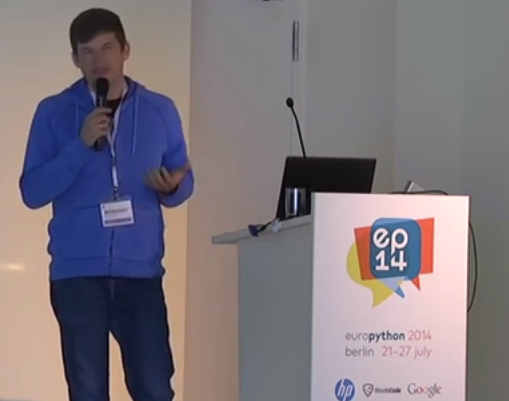
One of the most exciting applications of Social Media data is the automated identification, evaluation and prediction of trends. I already sketched some ideas in this blog post. Last year – and this was one of my personal highlights – I had the opportunity to speak at the PyData 2014 Berlin on the topic of Street Fighting Trend Research.

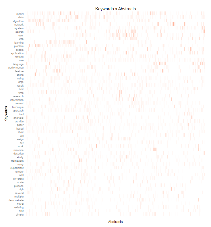
In my talk I presented some more general thoughts on trend research (or “coolhunting” as it is called nowadays) on the Internet. But at the core were three examples on how to identify research trends from the web (see this blogpost), how to mine conference proposals (see this analysis of Strata abstracts) and how to identify trending locations on Foursquare (see here). All three examples are also available as IPython Notebooks on my Github page. And here’s the recorded version of the talk.

The PyData conference was one of the best conferences I attended. Not only were the topics very diverse – ranging from GPU optimization to the representation of women in the PyData community – but also the people attending the conference were coming from different backgrounds: lawyers, engineers, physicists, computer scientists (of course) or statisticians. But still, with every talk and every conversation in the hallways, you could feel the wild euphoria connecting us all with the programming language and the incredible curiosity.

The Top 7 Beautiful Data Blog Posts in 2014

Domo_After2014 was a great year in data science – and also an exciting year for me personally from a very inspirational Strata Conference in Santa Clara to a wonderful experience of speaking at PyData Berlin to founding the data visualization company DataLion. But it also was a great year blogging about data science. Here’s the Beautiful Data blog posts our readers seemed to like the most:

  1. Datalicious Notebookmania – My personal list of the 7 IPython notebooks I like the most. Some of them are great for novices, some can even be challenging for advanced statisticians and datascientists
  2. Trending Topics at Strata Conferences 2011-2014 – An analysis of the topics most frequently mentioned in Strata Conference abstracts that clearly shows the rising importance of Python, IPython and Pandas.
  3. Big Data Investment Map 2014 – I’ve been tracking and analysing the developments in Big Data investments and IPOs for quite a long time. This was the 2014 update of the network mapping the investments of VCs in Big Data companies.
  4. Analyzing VC investment strategies with Crunchbase data – This blog post explains the code used to create the network.
  5. How to create a location graph from the Foursquare API – In this post, I explain a way to make sense out of the Foursquare API and to create geospatial network visualizations from the data showing how locations in a city are connected via Foursquare checkins.
  6. Text-Mining the DLD Conference 2014 – A very similar approach as I used for the Strata conference has been applied to the Twitter corpus refering to Hubert Burda Media DLD conference showing the trending topics in tech and media.
  7. Identifying trends in the German Google n-grams corpus – This tutorial shows how to analyze Big data-sets such as the Google Book ngram corpus with Hive on the Amazon Cloud.

Identifying trends in the German Google n-grams corpus (Tutorial)

A lot of people still have a lot of respect for Hadoop and MapReduce. I experience it regularly in workshops with market researchers and advertising people. Hadoop’s image is quite comparable with Linux’ perceived image in the 1990s: a tool for professional users that requires a lot of configuration. But in the same way, there were some user-friendly distributions (e.g. Suse), there are MapReduce tools that require almost no configuration.

One favorite example is the ease and speed, you can do serious analytical work on the Google n-grams corpus with Hive on Amazon’s Elastic MapReduce platform. I adapted the very helpful code from the AWS tutorial on the English corpus to find out the trending German words (or 1-grams) for the last century. You need to have an Amazon AWS account and valid SSH keys to connect to the machines you are running the MapReduce programs on (here’s the whole hive query file).

  • Start your Elastic MapReduce cluster on the EMR console. I used 1 Master and 19 slave nodes. Select your AWS ssh authorization key. Remember: from this moment on, your cluster is generating costs. So, don’t forget to terminate the cluster after the job is done!
  • If your Cluster has been set-up and is running, note the Master-Node-DNS. Open a SSH client (e.g. Putty on Windows or ssh on Linux) and connect to the master node with the ssh key. Your username on the remote machine is “hadoop”.
  • Start “hive” and set some useful defaults for the analytical job:

    set hive.base.inputformat=org.apache.hadoop.hive.ql.io.HiveInputFormat;
    set mapred.min.split.size=134217728;

  • The first code snippet connects to the 1-gram dataset which resides on the S3 storage:

    CREATE EXTERNAL TABLE german_1grams (
    gram string,
    year int,
    occurrences bigint,
    pages bigint,
    books bigint
    )
    ROW FORMAT DELIMITED FIELDS TERMINATED BY '\t'
    STORED AS SEQUENCEFILE
    LOCATION 's3://datasets.elasticmapreduce/ngrams/books/20090715/ger-all/1gram/';

  • Now, we can use this database to perform some operations. The first step is to normalize the database, e.g. to transform all words to lower case and remove 1-grams that are no proper words. Of course you could further refine this step to remove stopwords or reduce the words to their stems by stemming or lemmatization.

    CREATE TABLE normalized (
    gram string,
    year int,
    occurrences bigint
    );

    And then we populate this table:

    INSERT OVERWRITE TABLE normalized
    SELECT
    lower(gram),
    year,
    occurrences
    FROM
    german_1grams
    WHERE
    year >= 1889 AND
    gram REGEXP "^[A-Za-z+'-]+$";

  • The previous steps should run quite fast. Here’s the step that really need to be run on a multi-machine cluster:

    CREATE TABLE by_decade (
    gram string,
    decade int,
    ratio double
    );

    INSERT OVERWRITE TABLE by_decade
    SELECT
    a.gram,
    b.decade,
    sum(a.occurrences) / b.total
    FROM
    normalized a
    JOIN (
    SELECT
    substr(year, 0, 3) as decade,
    sum(occurrences) as total
    FROM
    normalized
    GROUP BY
    substr(year, 0, 3)
    ) b
    ON
    substr(a.year, 0, 3) = b.decade
    GROUP BY
    a.gram,
    b.decade,
    b.total;

  • The final step is to count all the trending words and export the data:

    CREATE TABLE result_decade (
    gram string,
    decade int,
    ratio double,
    increase double );

    INSERT OVERWRITE TABLE result_decade
    SELECT
    a.gram as gram,
    a.decade as decade,
    a.ratio as ratio,
    a.ratio / b.ratio as increase
    FROM
    by_decade a
    JOIN
    by_decade b
    ON
    a.gram = b.gram and
    a.decade - 1 = b.decade
    WHERE
    a.ratio > 0.000001 and
    a.decade >= 190
    DISTRIBUTE BY
    decade
    SORT BY
    decade ASC,
    increase DESC;

  • The result is saved as a tab delimited plaintext data file. We just have to find out its correct location and then transfer it from the Hadoop HDFS file system to the “normal” file system on the remote machine and then transfer it to our local computer. The (successful) end of the hive job should look like this on your ssh console:
    EMR_finish
    The line “Deleted hdfs://x.x.x.x:9000/mnt/hive_0110/warehouse/export” gives you the information where the file is located. You can transfer it with the following command:

    $ hdfs dfs -cat /mnt/hive_0110/warehouse/export/* > ~/export_file.txt

  • Now the data is in the home directory of the remote hadoop user in the file export_file.txt. With a secure file copy program such as scp or WinSCP you can download the file to your local machine. On a Linux machine, I should have converted the AWS SSH key in the Linux format (id_rsa and id_rsa.pub) and then added. With the following command I could download our results (replace x.x.x.x with your IP address or the Master-Host-DNS):

    $ scp your_username@x.x.x.x:export_file.txt ~/export_file.txt

  • After you verified that the file is intact, you can terminate your Elastic MapReduce instances.

As a result you get a large text file with information on the ngram, decade, relative frequency and growth ratio in comparison with the previous decade. After converting this file into a more readable Excel document with this Python program, it looks like this:
ngrams_results

Values higher than 1 in the increase column means that this word has grown in importance while values lower than 1 means that this word had been used more frequently in the previous decade.

Here’s the top 30 results per decade:

  • 1900s: Adrenalin, Elektronentheorie, Textabb, Zysten, Weininger, drahtlosen, Mutterschutz, Plazenta, Tonerde, Windhuk, Perseveration, Karzinom, Elektrons, Leukozyten, Housz, Schecks, kber, Zentralwindung, Tarifvertrags, drahtlose, Straftaten, Anopheles, Trypanosomen, radioaktive, Tonschiefer, Achsenzylinder, Heynlin, Bastimento, Fritter, Straftat
  • 1910s: Commerzdeputation, Bootkrieg, Diathermie, Feldgrauen, Sasonow, Wehrbeitrag, Bolschewismus, bolschewistischen, Porck, Kriegswirtschaft, Expressionismus, Bolschewiki, Wirtschaftskrieg, HSM, Strahlentherapie, Kriegsziele, Schizophrenie, Berufsberatung, Balkankrieg, Schizophrenen, Enver, Angestelltenversicherung, Strahlenbehandlung, Orczy, Narodna, EKG, Besenval, Flugzeugen, Flugzeuge, Wirkenseinheit
  • 1920s: Reichsbahngesellschaft, Milld, Dawesplan, Kungtse, Fascismus, Eidetiker, Spannungsfunktion, Paneuropa, Krestinski, Orogen, Tschechoslovakischen, Weltwirtschaftskonferenz, RSFSR, Sachv, Inflationszeit, Komintern, UdSSR, RPF, Reparationszahlungen, Sachlieferungen, Konjunkturforschung, Schizothymen, Betriebswirtschaftslehre, Kriegsschuldfrage, Nachkriegsjahre, Mussorgski, Nachkriegsjahren, Nachkriegszeit, Notgemeinschaft, Erlik
  • 1930s: Reichsarbeitsdienst, Wehrwirtschaft, Anerbengericht, Remilitarisierung, Steuergutscheine, Huguenau, Molotov, Volksfront, Hauptvereinigung, Reichsarbeitsdienstes, Viruses, Mandschukuo, Erzeugungsschlacht, Neutrons, MacHeath, Reichsautobahnen, Ciano, Vierjahresplan, Erbkranken, Schuschnigg, Reichsgruppe, Arbeitsfront, NSDAP, Tarifordnungen, Vierjahresplanes, Mutationsrate, Erbhof, GDI, Hitlerjugend, Gemeinnutz
  • 1940s: KLV, Cibazol, UNRRA, Vollziehungsrath, Bhil, Verordening, Akha, Sulfamides, Ekiken, Wehrmachtbericht, Capsiden, Meau, Lewerenz, Wehrmachtsbericht, juedischen, Kriegsberichter, Rourden, Gauwirtschaftskammer, Kriegseinsatz, Bidault, Sartre, Riepp, Thailands, Oppanol, Jeftanovic, OEEC, Westzonen, Secretaris, pharmaceutiques, Lodsch
  • 1950s: DDZ, Peniteat, ACTH, Bleist, Siebenjahrplan, Reaktoren, Cortison, Stalinallee, Betriebsparteiorganisation, Europaarmee, NPDP, SVN, Genossenschaftsbauern, Grundorganisationen, Sputnik, Wasserstoffwaffen, ADAP, BverfGg, Chruschtschows, Abung, CVP, Atomtod, Chruschtschow, Andagoya, LPG, OECE, LDPD, Hakoah, Cortisone, GrundG
  • 1960s: Goldburg, Dubcek, Entwicklungszusammenarbeit, Industriepreisreform, Thant, Hoggan, Rhetikus, NPD, Globalstrategie, Notstandsgesetze, Nichtverbreitung, Kennedys, PPF, Pompidou, Nichtweiterverbreitung, neokolonialistischen, Teilhards, Notstandsverfassung, Biafra, Kiesingers, McNamara, Hochhuth, BMZ, OAU, Dutschke, Rusk, Neokolonialismus, Atomstreitmacht, Periodikums, MLF
  • 1970s: Zsfassung, Eurokommunismus, Labov, Sprechakttheorie, Werkkreis, Uerden, Textsorte, NPS, Legitimationsprobleme, Aktanten, Kurztitelaufnahme, Parlamentsfragen, Textsorten, Soziolinguistik, Rawls, Uird, Textlinguistik, IPW, Positivismusstreit, Jusos, UTB, Komplexprogramms, Praxisbezug, performativen, Todorov, Namibias, Uenn, ZSta, Energiekrise, Lernzielen
  • 1980s: Gorbatschows, Myanmar, Solidarnosc, FMLN, Schattenwirtschaft, Gorbatschow, Contadora, Sandinisten, Historikerstreit, Reagans, sandinistische, Postmoderne, Perestrojka, BTX, Glasnost, Zeitzeugen, Reagan, Miskito, nicaraguanischen, Madeyski, Frauenforschung, FSLN, sandinistischen, Contras, Lyotard, Fachi, Gentechnologie, UNIX, Tschernobyl, Beijing
  • 1990s: BSTU, Informationsamt, Sapmo, SOEP, Tschetschenien, EGV, BMBF, OSZE, Zaig, Posllach, Oibe, Benchmarking, postkommunistischen, Reengineering, Gauck, Osterweiterung, Belarus, Tatarstan, Beitrittsgebiet, Cyberspace, Goldhagens, Treuhandanstalt, Outsourcing, Modrows, Diensteinheiten, EZB, Einigungsvertrages, Einigungsvertrag, Wessis, Einheitsaufnahme
  • 2000s: MySQL, Servlet, Firefox, LFRS, Dreamweaver, iPod, Blog, Weblogs, VoIP, Weblog, Messmodells, Messmodelle, Blogs, Mozilla, Stylesheet, Nameserver, Google, Markenmanagement, JDBC, IPSEC, Bluetooth, Offshoring, ASPX, WLAN, Wikipedia, Messmodell, Praxistipp, RFID, Grin, Staroffice

Street Fighting Trend Research

One of the most intriguing tools for the Street Fighting Data Science approach is the new Google Trends interface (formerly known as Google Insights for Search). This web application allows to analyze the volume of search requests for particular keywords over time (from 2004 on). This can be very useful for evaluating product life-cycle – assuming a product or brand that is not being searched on Google is no longer relevant. Here’s the result for the most important products in the Samsung Galaxy range:

For the S3 and S4 model the patterns are almost the same:

  • Stage 1: a slow build-up starting in the moment on the product was first mentioned in the Internet
  • Stage 2: a sudden burst at the product launch
  • Stage 3: a plateau phase with additional spikes when product modifications are launched
  • Stage 4: a slow decay of attention when other products have appeared

The S2 on the other hand does not have this sudden burst at launch while the Galaxy Note does not decay yet but displays multiple bursts of attention.

But in South Korea, the cycles seem quite different:

If you take a look at the relative numbers, the Galaxy Note is much stronger in South Korea and at the moment is at no. 1 of the products examined.

An interesting question is: do these patterns also hold for other mobile / smartphone brands? Here’s a look at the iPhone generations as searched for by Google users:

The huge spike at the launch of the iPhone 5 hints at the most successful launch in terms of Google attention. But this doesn’t say anything about the sentiment of the attention. Interestingly enough, the iPhone 5 had a first burst at the same moment the iPhone 4S has been launched. The reason for this anomany: people were expecting that Apple would be launching the iPhone 5 in Sep/Oct 2011 but then were disappointed that the Cupertino launch event was only about a iPhone 4S.

Analyses like this are especially useful at the beginning of a trend research workflow. The next steps would involve digging deeper in the patterns, taking a look at the audiences behind the data, collecting posts, tweets and news articles for the peaks in the timelines, looking for correlations of the timelines in other data sets e.g. with Google Correlate, brand tracking data or consumer surveys.

Mining Research Interests – or: What Would Google Want to Know?

I am a regular visitor of Google’s research page where they post all of their latest and upcoming scientific papers. Lately I have thought whether it would be possible to statistically extract some of the meta-information from the papers. Here’s the result of the analysis of the papers’ titles produced with just a few lines of R code:

Research Topics @ Google


I clustered the data with a standard hierarchical cluster analysis to find out which terms tend to often go together in the paper titles. Then I took a deeper look at the abstracts – of all the papers that had abstracts that is. I processed the abstracts with the tm R package and draw the following heat-map that shows how often which of the most important keywords appear in each paper:

Keywords_Abstracts_google

I did a similar heatmap but this time normalized by the term frequency – inverse document frequency measure. While the first heatmap shows the most frequently used terms, this weighted heatmap shows terms that are quite important in their respective research papers but normalizes this by the overall term frequency.

Keywords_Abstracts_google_tfidf

If you need input for playing buzzword bingo at the next Strata Conference in Santa Clara, you don’t have to look any further 😉