2014 highlight (2): On of the best courses on Big Data and Data Mining

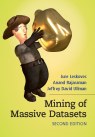
I already mentioned the Hastie & Tibshirani course on statistical learning as one of my personal highlights in data science last year. My second highlight is also an online course, also by leading experts on their field (this time: Big Data and data mining), also based on a (freely available) book and also by Stanford University professors: Jure Leskovec, Anand Rajamaran and Jeff Ullman’s course on “Mining Massive Datasets”.

ullman_mmds

If you’re interested in data science or data mining, chances are high that you have already been in touch with their book. It can safely be considered a standard work on the fascinating intersection of data mining algorithms, machine learning and Big Data. The 7 week course is the online version of the Stanford courses CS246 and the earlier version of CS345A.

mmds_cover_v21The course is very dense and covers a lot of territory from the book, for example:

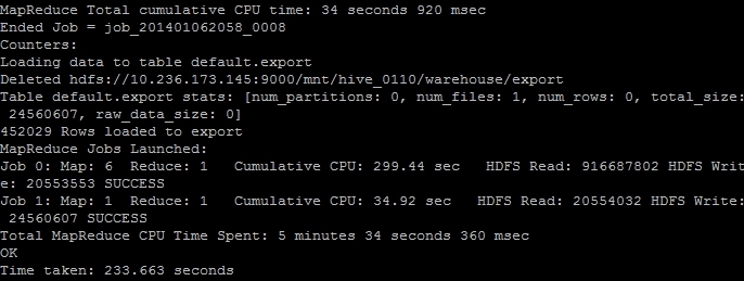
  • How does Map Reduce work and why is it important?
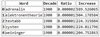
  • How can I retrieve frequently appearing combinations from very large sets of items such as shopping baskets?
  • How to retain information about a datastream that does not fit in memory?
  • What are the most common tasks in supervised machine learning and how to implement them?
  • How do I program an intelligent system for recommending movies?
  • How to compute optimal placements of online advertisements?

Some of the lectures are on a beginners to intermediate level, but some lectures cover very advanced topics. What I especially liked about this course is that a lot of the material covered really is state-of-the-art in data mining. Some algorithms – e.g. the BIGCLAM community detection and CUR matrix decomposition – had only been developed about year ago.

So, take a look at the book, and if you haven’t already: enroll at the Coursera course website to make sure you won’t miss the next session of this course.

The Top 7 Beautiful Data Blog Posts in 2014

Domo_After2014 was a great year in data science – and also an exciting year for me personally from a very inspirational Strata Conference in Santa Clara to a wonderful experience of speaking at PyData Berlin to founding the data visualization company DataLion. But it also was a great year blogging about data science. Here’s the Beautiful Data blog posts our readers seemed to like the most:

  1. Datalicious Notebookmania – My personal list of the 7 IPython notebooks I like the most. Some of them are great for novices, some can even be challenging for advanced statisticians and datascientists
  2. Trending Topics at Strata Conferences 2011-2014 – An analysis of the topics most frequently mentioned in Strata Conference abstracts that clearly shows the rising importance of Python, IPython and Pandas.
  3. Big Data Investment Map 2014 – I’ve been tracking and analysing the developments in Big Data investments and IPOs for quite a long time. This was the 2014 update of the network mapping the investments of VCs in Big Data companies.
  4. Analyzing VC investment strategies with Crunchbase data – This blog post explains the code used to create the network.
  5. How to create a location graph from the Foursquare API – In this post, I explain a way to make sense out of the Foursquare API and to create geospatial network visualizations from the data showing how locations in a city are connected via Foursquare checkins.
  6. Text-Mining the DLD Conference 2014 – A very similar approach as I used for the Strata conference has been applied to the Twitter corpus refering to Hubert Burda Media DLD conference showing the trending topics in tech and media.
  7. Identifying trends in the German Google n-grams corpus – This tutorial shows how to analyze Big data-sets such as the Google Book ngram corpus with Hive on the Amazon Cloud.

Trending Topics at Strata Conferences 2011-2014

To fill the gap until this year’s Strata Conference in Santa Clara, I thought of a way to find out trends in big data and data science. As this conference should easily be the leading edge gathering of practitioners, theorists and followers of big data analytics, the abstracts submitted and accepted for Strataconf should give some valuable input. So, I collected the abstracts from the last Santa Clara Strata conferences and applied some Python nltk magic to it – all in a single IPython Notebook, of course.

Here’s a look at the resulting insights. First, I analyzed the most frequent words, people used in their abstracts (after excluding common English language stop words). As a starter, here’s the Top 20 words for the last four Strata conferences:

Strata_Words_2011 Strata_Words_2012 Strata_Words_2013 Strata_Words_2014

This is just to check, whether all the important buzzwords are there and we’re measuring the right things here: Data – check! Hadoop – check! Big – check! Business – check! Already with this simple frequency count, one thing seems very interesting: Hadoop didn’t seem to be a big topic in the community until 2012. Another random conclusion could be that 2011 was the year where Big Data really was “new”. This word loses traction in the following years.

And now for something a bit more sophisticated: Bigrams or frequently used word combinations:

2011
Strata_Bigrams_2011
2012
Strata_Bigrams_2012
2013
Strata_Bigrams_2013
2014
Strata_Bigrams_2014

Of course, the top bigram through all the years is “big data”, which is not entirely unexpected. But you can clearly see some variation among the Top 20. Looking at the relative frequency of the mentions, you can see that the most important topic “Big Data” will probably not be as important in this years conference – the topical variety seems to be increasing:

Strata_Bigrams

Looking at some famous programming and mathematical languages, the strong dominance of R seems to be broken by Python or IPython (and its Notebook environment) which seems to have established itself as the ideal programming tool for the nerdy real-time presentation of data hacks. \o/

Strata_Lang

Another trend can be seen in the following chart: Big Data seems to become more and more faceted over the years. The dominant focus on business applications of data analysis seems to be over and the number of different topics discussed on the conference seems to be increasing:

Strata_Fields

Finally, let’s take a more systematic look at rising topics at Strata Conferences. To find out which topics were gaining momentum, I calculated the relative frequencies of all the words and compared them to the year before. So, here’s the trending topics:

Strata_Trends_2012 Strata_Trends_2013 Strata_Trends_2014

These charts show that 2012 was indeed the “Hadoop-Strata” where this technology was the great story for the community, but also the programming language R became the favorite Swiss knife for data scientists. 2013 was about applications like Hive that run on top of Hadoop, data visualizations and Google seemed to generate a lot of buzz in the community. Also, 2013 was the year, data really became a science – this is the second most important trending topic. And this was exactly the way, I experienced the 2013 Strata “on the ground” in Santa Clara.

What will 2014 bring? The data suggests, it will be the return of the hardware (e.g. high performance clusters), but also about building data architectures, bringing data know-how into organizations and on a more technical dimension about graph processing. Sounds very promising in my ears!

Identifying trends in the German Google n-grams corpus (Tutorial)

A lot of people still have a lot of respect for Hadoop and MapReduce. I experience it regularly in workshops with market researchers and advertising people. Hadoop’s image is quite comparable with Linux’ perceived image in the 1990s: a tool for professional users that requires a lot of configuration. But in the same way, there were some user-friendly distributions (e.g. Suse), there are MapReduce tools that require almost no configuration.

One favorite example is the ease and speed, you can do serious analytical work on the Google n-grams corpus with Hive on Amazon’s Elastic MapReduce platform. I adapted the very helpful code from the AWS tutorial on the English corpus to find out the trending German words (or 1-grams) for the last century. You need to have an Amazon AWS account and valid SSH keys to connect to the machines you are running the MapReduce programs on (here’s the whole hive query file).

  • Start your Elastic MapReduce cluster on the EMR console. I used 1 Master and 19 slave nodes. Select your AWS ssh authorization key. Remember: from this moment on, your cluster is generating costs. So, don’t forget to terminate the cluster after the job is done!
  • If your Cluster has been set-up and is running, note the Master-Node-DNS. Open a SSH client (e.g. Putty on Windows or ssh on Linux) and connect to the master node with the ssh key. Your username on the remote machine is “hadoop”.
  • Start “hive” and set some useful defaults for the analytical job:

    set hive.base.inputformat=org.apache.hadoop.hive.ql.io.HiveInputFormat;
    set mapred.min.split.size=134217728;

  • The first code snippet connects to the 1-gram dataset which resides on the S3 storage:

    CREATE EXTERNAL TABLE german_1grams (
    gram string,
    year int,
    occurrences bigint,
    pages bigint,
    books bigint
    )
    ROW FORMAT DELIMITED FIELDS TERMINATED BY '\t'
    STORED AS SEQUENCEFILE
    LOCATION 's3://datasets.elasticmapreduce/ngrams/books/20090715/ger-all/1gram/';

  • Now, we can use this database to perform some operations. The first step is to normalize the database, e.g. to transform all words to lower case and remove 1-grams that are no proper words. Of course you could further refine this step to remove stopwords or reduce the words to their stems by stemming or lemmatization.

    CREATE TABLE normalized (
    gram string,
    year int,
    occurrences bigint
    );

    And then we populate this table:

    INSERT OVERWRITE TABLE normalized
    SELECT
    lower(gram),
    year,
    occurrences
    FROM
    german_1grams
    WHERE
    year >= 1889 AND
    gram REGEXP "^[A-Za-z+'-]+$";

  • The previous steps should run quite fast. Here’s the step that really need to be run on a multi-machine cluster:

    CREATE TABLE by_decade (
    gram string,
    decade int,
    ratio double
    );

    INSERT OVERWRITE TABLE by_decade
    SELECT
    a.gram,
    b.decade,
    sum(a.occurrences) / b.total
    FROM
    normalized a
    JOIN (
    SELECT
    substr(year, 0, 3) as decade,
    sum(occurrences) as total
    FROM
    normalized
    GROUP BY
    substr(year, 0, 3)
    ) b
    ON
    substr(a.year, 0, 3) = b.decade
    GROUP BY
    a.gram,
    b.decade,
    b.total;

  • The final step is to count all the trending words and export the data:

    CREATE TABLE result_decade (
    gram string,
    decade int,
    ratio double,
    increase double );

    INSERT OVERWRITE TABLE result_decade
    SELECT
    a.gram as gram,
    a.decade as decade,
    a.ratio as ratio,
    a.ratio / b.ratio as increase
    FROM
    by_decade a
    JOIN
    by_decade b
    ON
    a.gram = b.gram and
    a.decade - 1 = b.decade
    WHERE
    a.ratio > 0.000001 and
    a.decade >= 190
    DISTRIBUTE BY
    decade
    SORT BY
    decade ASC,
    increase DESC;

  • The result is saved as a tab delimited plaintext data file. We just have to find out its correct location and then transfer it from the Hadoop HDFS file system to the “normal” file system on the remote machine and then transfer it to our local computer. The (successful) end of the hive job should look like this on your ssh console:
    EMR_finish
    The line “Deleted hdfs://x.x.x.x:9000/mnt/hive_0110/warehouse/export” gives you the information where the file is located. You can transfer it with the following command:

    $ hdfs dfs -cat /mnt/hive_0110/warehouse/export/* > ~/export_file.txt

  • Now the data is in the home directory of the remote hadoop user in the file export_file.txt. With a secure file copy program such as scp or WinSCP you can download the file to your local machine. On a Linux machine, I should have converted the AWS SSH key in the Linux format (id_rsa and id_rsa.pub) and then added. With the following command I could download our results (replace x.x.x.x with your IP address or the Master-Host-DNS):

    $ scp your_username@x.x.x.x:export_file.txt ~/export_file.txt

  • After you verified that the file is intact, you can terminate your Elastic MapReduce instances.

As a result you get a large text file with information on the ngram, decade, relative frequency and growth ratio in comparison with the previous decade. After converting this file into a more readable Excel document with this Python program, it looks like this:
ngrams_results

Values higher than 1 in the increase column means that this word has grown in importance while values lower than 1 means that this word had been used more frequently in the previous decade.

Here’s the top 30 results per decade:

  • 1900s: Adrenalin, Elektronentheorie, Textabb, Zysten, Weininger, drahtlosen, Mutterschutz, Plazenta, Tonerde, Windhuk, Perseveration, Karzinom, Elektrons, Leukozyten, Housz, Schecks, kber, Zentralwindung, Tarifvertrags, drahtlose, Straftaten, Anopheles, Trypanosomen, radioaktive, Tonschiefer, Achsenzylinder, Heynlin, Bastimento, Fritter, Straftat
  • 1910s: Commerzdeputation, Bootkrieg, Diathermie, Feldgrauen, Sasonow, Wehrbeitrag, Bolschewismus, bolschewistischen, Porck, Kriegswirtschaft, Expressionismus, Bolschewiki, Wirtschaftskrieg, HSM, Strahlentherapie, Kriegsziele, Schizophrenie, Berufsberatung, Balkankrieg, Schizophrenen, Enver, Angestelltenversicherung, Strahlenbehandlung, Orczy, Narodna, EKG, Besenval, Flugzeugen, Flugzeuge, Wirkenseinheit
  • 1920s: Reichsbahngesellschaft, Milld, Dawesplan, Kungtse, Fascismus, Eidetiker, Spannungsfunktion, Paneuropa, Krestinski, Orogen, Tschechoslovakischen, Weltwirtschaftskonferenz, RSFSR, Sachv, Inflationszeit, Komintern, UdSSR, RPF, Reparationszahlungen, Sachlieferungen, Konjunkturforschung, Schizothymen, Betriebswirtschaftslehre, Kriegsschuldfrage, Nachkriegsjahre, Mussorgski, Nachkriegsjahren, Nachkriegszeit, Notgemeinschaft, Erlik
  • 1930s: Reichsarbeitsdienst, Wehrwirtschaft, Anerbengericht, Remilitarisierung, Steuergutscheine, Huguenau, Molotov, Volksfront, Hauptvereinigung, Reichsarbeitsdienstes, Viruses, Mandschukuo, Erzeugungsschlacht, Neutrons, MacHeath, Reichsautobahnen, Ciano, Vierjahresplan, Erbkranken, Schuschnigg, Reichsgruppe, Arbeitsfront, NSDAP, Tarifordnungen, Vierjahresplanes, Mutationsrate, Erbhof, GDI, Hitlerjugend, Gemeinnutz
  • 1940s: KLV, Cibazol, UNRRA, Vollziehungsrath, Bhil, Verordening, Akha, Sulfamides, Ekiken, Wehrmachtbericht, Capsiden, Meau, Lewerenz, Wehrmachtsbericht, juedischen, Kriegsberichter, Rourden, Gauwirtschaftskammer, Kriegseinsatz, Bidault, Sartre, Riepp, Thailands, Oppanol, Jeftanovic, OEEC, Westzonen, Secretaris, pharmaceutiques, Lodsch
  • 1950s: DDZ, Peniteat, ACTH, Bleist, Siebenjahrplan, Reaktoren, Cortison, Stalinallee, Betriebsparteiorganisation, Europaarmee, NPDP, SVN, Genossenschaftsbauern, Grundorganisationen, Sputnik, Wasserstoffwaffen, ADAP, BverfGg, Chruschtschows, Abung, CVP, Atomtod, Chruschtschow, Andagoya, LPG, OECE, LDPD, Hakoah, Cortisone, GrundG
  • 1960s: Goldburg, Dubcek, Entwicklungszusammenarbeit, Industriepreisreform, Thant, Hoggan, Rhetikus, NPD, Globalstrategie, Notstandsgesetze, Nichtverbreitung, Kennedys, PPF, Pompidou, Nichtweiterverbreitung, neokolonialistischen, Teilhards, Notstandsverfassung, Biafra, Kiesingers, McNamara, Hochhuth, BMZ, OAU, Dutschke, Rusk, Neokolonialismus, Atomstreitmacht, Periodikums, MLF
  • 1970s: Zsfassung, Eurokommunismus, Labov, Sprechakttheorie, Werkkreis, Uerden, Textsorte, NPS, Legitimationsprobleme, Aktanten, Kurztitelaufnahme, Parlamentsfragen, Textsorten, Soziolinguistik, Rawls, Uird, Textlinguistik, IPW, Positivismusstreit, Jusos, UTB, Komplexprogramms, Praxisbezug, performativen, Todorov, Namibias, Uenn, ZSta, Energiekrise, Lernzielen
  • 1980s: Gorbatschows, Myanmar, Solidarnosc, FMLN, Schattenwirtschaft, Gorbatschow, Contadora, Sandinisten, Historikerstreit, Reagans, sandinistische, Postmoderne, Perestrojka, BTX, Glasnost, Zeitzeugen, Reagan, Miskito, nicaraguanischen, Madeyski, Frauenforschung, FSLN, sandinistischen, Contras, Lyotard, Fachi, Gentechnologie, UNIX, Tschernobyl, Beijing
  • 1990s: BSTU, Informationsamt, Sapmo, SOEP, Tschetschenien, EGV, BMBF, OSZE, Zaig, Posllach, Oibe, Benchmarking, postkommunistischen, Reengineering, Gauck, Osterweiterung, Belarus, Tatarstan, Beitrittsgebiet, Cyberspace, Goldhagens, Treuhandanstalt, Outsourcing, Modrows, Diensteinheiten, EZB, Einigungsvertrages, Einigungsvertrag, Wessis, Einheitsaufnahme
  • 2000s: MySQL, Servlet, Firefox, LFRS, Dreamweaver, iPod, Blog, Weblogs, VoIP, Weblog, Messmodells, Messmodelle, Blogs, Mozilla, Stylesheet, Nameserver, Google, Markenmanagement, JDBC, IPSEC, Bluetooth, Offshoring, ASPX, WLAN, Wikipedia, Messmodell, Praxistipp, RFID, Grin, Staroffice