What I really love about Twitter is that everything they do seems to be data-based. They’re so data-driven, they even analyze the ingredients of their lunch to ensure everyone at the company is living a healthy lifestyle. So, the decision for Berlin as their German headquarter cannot be a random or value-based decision. I bet, there’s been a lot of numbers crunching before announcing their new office. Let’s try and reverse-engineer this decision.
As a data basis I collected 4,377,832 tweets more or less randomly by connecting to the streaming API. Then I pulled all users mentioning one of the 30 leading German cities from Berlin to Aachen in their location field. Where there were Umlauts involved, I allowed for multiple variants, e.g. “Muenchen”, “Munchen” or “Munich” for “München”. Now I have 3,696 Twitter users from Germany that posted one or more tweets during the sample interval. That’s 0.08% of the original sample size. Although that’s not as much as I would have expected, let’s continue with the analysis.
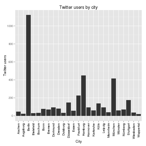
The first interesting thing is the distribution of the Twitter users by their cities. Here’s the result:
One thing should immediately be clear from this chart: Only Berlin, Hamburg and Munich had a real chance of becoming Twitter’s German HQ. The other cities are just Twitter ghost towns. In the press, there had been some buzz about Cologne, but from these numbers, I’d say that could only have been desinformation or whishful thinking.
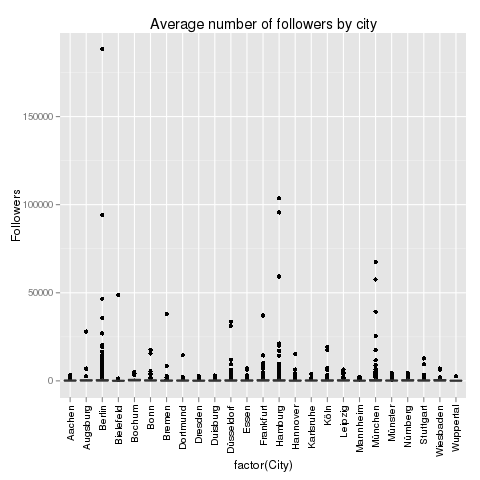
The next thing to look at is the influence of Twitter users in different German cities. Here’s a look at the follower data:
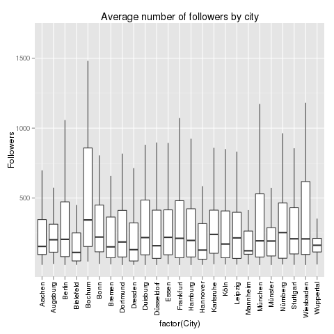
This does not help a lot. The distribution is heavily distorted by the outliers: Some Twitter users have a lot more followers than others. These Twitter users are marked by the black dots above the cities. But one thing is interesting: Berlin, Hamburg and Munich not only have the most Twitter users in our sample, but also the most and the highest outliers. With the outliers removed, the chart looks like this:
The chart not only shows the median number of followers, but also the distribution of the data. Berlin, that should be clear from this chart, is not the German city where the Twitter users with most followers hail from. This should be awarded to Bochum (355 followers), Nuremberg (258 followers) or Augsburg (243 followers). But these numbers are not very reliable as the number of cases is quite low for these cities. If we focus on the Big 3, then Berlin is leading with 223 followers, then Munich with 209 followers and finally Hamburg with 200 followers. But it’s a very close race.
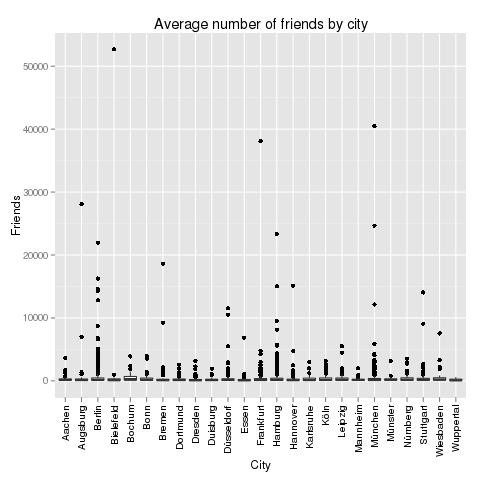
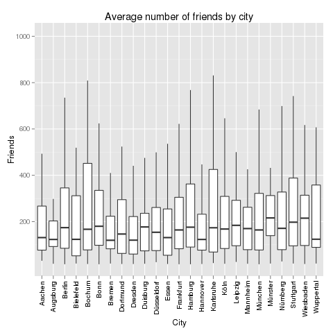
Next up, the number of friends. Which German city is leading the average number of friends on Twitter?
This chart is also distorted by outliers, but here it’s different cities: The user in the sample who is following the largest number of friends is located in Bielefeld. Of all things! Now, let’s remove the outliers:
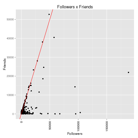
The cities with the larges average number of friends are: Bochum (again! 286 friends), Wiesbaden (224 friends) and Leipzig (208 friends). Our Big 3 are performing as follows: Berlin (183 friends), Hamburg (183 friends) and Munich (160 friends). Let’s take a look at the relation between followers and friends:
If we zoom in a bit on the data we can reproduce the “2000 phenomenon”:
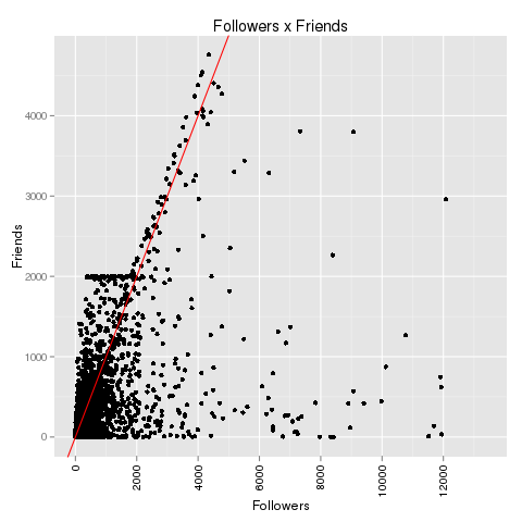
There clearly is some kind of artificial barrier at 2,000 friends on Twitter. Accounts that have between 100 and 2,000 followers never follow more than 2,000 followers. Most frequently, they follow just a little below of 2,000 people. After they gathered 2,000 followers themselves, this barrier has been broken and the maximal number of friends seems to grow with the number of followers. There’s only speculation about this phenomenon, but one of the most convincing explanation is: We are looking at spam bots that are programmed to stay below 2,000 friends until they have gathered more than 2,000 followers. Maybe Twitter has some spam fighting algorithms that are focusing at the 2,000 line. Update: See explanation in the comments to this article: Behind this anomaly is Twitter’s spam-fighting barrier that only allows 2,000 friends up to 2,000 followers. Beyond this, the limit for the maximum number of friends is limited by the number of followers + 10%.
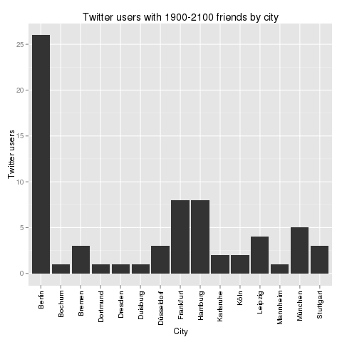
If those users are bots, then which city is bot capital? Let’s take a look at all Twitter users that have between 1,900 and 2,100 friends and segment them by city:
Again, Berlin is leading. But how do these numbers relate to the total numbers? Here’s the Bot Score for these cities: Berlin 2.3%, Hamburg 1.8% and Munich 1.2%. That’s one clear point for Munich.
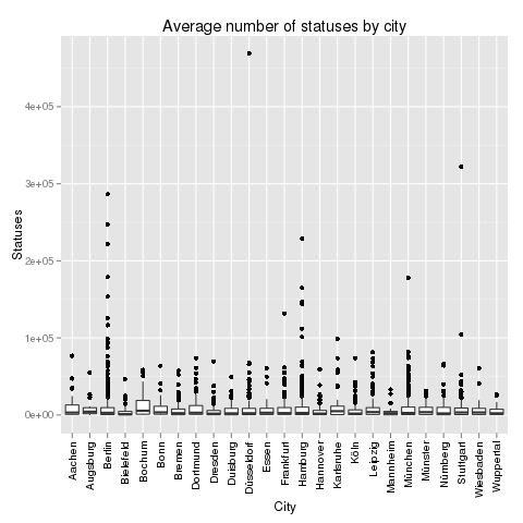
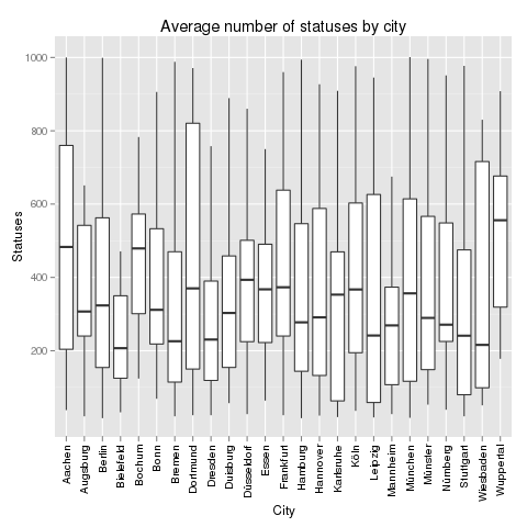
Finally, let’s take a look at Twitter statuses in these cities. Where do the most active Twitter users tweet from? Here’s a look at the full picture including outliers:
The city with the most active Twitter user surprisingly is not Bochum or Berlin, but Düsseldorf. And also Stuttgart seems to be very hot in this regard. But to really learn about activity, we have to remove the outliers again:
Without outliers, the most active Twitter cities in Germany are: Bochum (again!! 5514 statuses), Karlsruhe (4973) and Augsburg (4254). The Big 3 are in the midfield: Berlin (2845), Munich (2717) and Hamburg (2638).
Finally, there’s always the content. What are the users in the Big 3 cities talking about? The most frequently twittered words do not differ very much. In all three cities, “RT” is the most important word followed by a lot of words like “in”, “the” or “ich” that don’t tell much about the topics. It is much more interesting to look at word pairs (and especially at the pairs with the highest point wise mutual information (PMI). In Berlin, people are talking about “neues Buch” (new book – it’s a city of literature), “gangbang erotik” (hmm) and “nasdaq dow” (financial information seem to be important). In Munich, it’s “reise reisen” (Munich seems to love traveling), “design products” (very design oriented city) and “prost bier” (it’s a cliche, but it seems to be true). Compare this with Hamburg’s “amazon preis” (people looking for low prices), “social media” (Hamburg has a lot of online agencies) and “dvd blueray” (people watching a lot of TV).
Wrapping up, here are the final results:
          Berlin Munich Hamburg
Users          3      1       2
Followers      3      2       1
Friends        2      1       2
Bots          -3     -1      -2
Statuses       3      2       1
TOTAL          8      5       4
Congrats to Berlin!
[The R code that generated all the charts above can be found on my github.]

